Quantitative Finance
The Black-Scholes Model: Derivations, Assumptions, and Limitations
Understand the mathematical foundations of the 1973 Nobel-prize winning model and why fat tails cause real-world deviations.
📅 28 August 2026•⏱️ 8 min read•✍️ OptionPricing Quantitative Team
Share:
📢 Share this Quantitative Guide:
📌 Key Takeaways
- ✓Black-Scholes (1973) established closed-form differential equations for pricing European options.
- ✓Assumes geometric Brownian motion, lognormal return distribution, and constant volatility.
- ✓Real-world market fat tails (kurtosis) cause out-of-the-money options to deviate from theory.
- ✓Modern pricing engines adjust Black-Scholes outputs using implied volatility surfaces.
📖 Table of Contents
1. The Partial Differential Equation
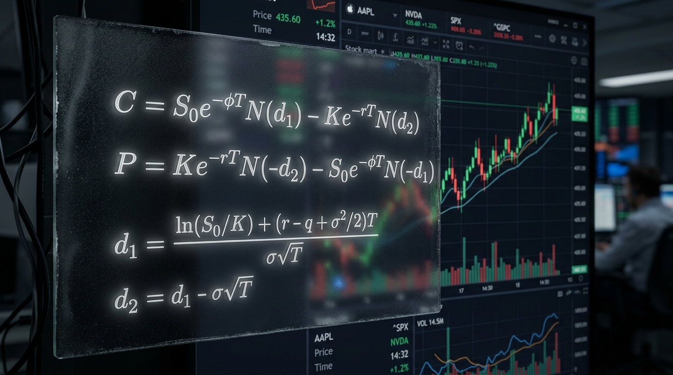
Fischer Black, Myron Scholes, and Robert Merton derived a partial differential equation governing the price of a derivative under geometric Brownian motion:
∂V/∂t + ½σ²S²(∂²V/∂S²) + rS(∂V/∂S) - rV = 0
2. Theoretical Model Assumptions
- European-style exercise (only at expiration date T).
- Constant volatility σ and risk-free interest rate r.
- Zero transaction costs and continuous trading liquidity.
- Lognormal distribution of underlying asset returns.
3. Real-World Market Limitations
Actual market asset returns exhibit "fat tails" (excess kurtosis) — extreme price shocks occur more frequently than predicted by a standard bell curve. Quantitative desks adjust Black-Scholes using implied volatility surfaces.
Found this quantitative guide helpful?Share it with fellow option traders and financial analysts.
📜 In This Article
Try Option Pricing Tools Live
Calculate Black-Scholes theoretical prices, Greeks, and multi-leg strategy payoffs instantly in your browser.
Open Black-Scholes Pricer →